Performance Reports & Analysis IFU042(04)

Performance Reports Management

The Performance Reports Management page is the Data Analysis entry point for generated Performance Reports in the RARE portal. It helps LF manufacturing, quality and laboratory science users review how an assay configuration performs against known reference data, and provides the audit trail needed to understand exactly which dataset, classifier, batch configuration, software version and report configuration produced a given result.

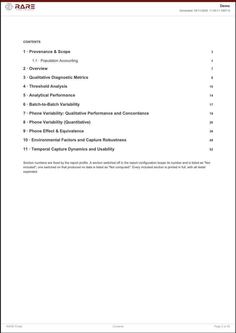
The generated report layout uses a fixed 11-section structure. Sections that are switched off keep their section number in the contents, while included sections are printed in full.

Why use Performance Reports?

A Performance Report acts as a snapshot in time. It records how a specific dataset performed with a specific version of the qualitative classifier, quantitative batch configuration and report settings.

This is useful for:

• Method validation and design history evidence: capturing the diagnostic and analytical metrics used to support performance claims.

• Configuration tuning: comparing thresholds, classifiers, calibration curves and report limits before fixing an operating configuration.

• Manufacturing and QC review: checking lot-to-lot consistency, concentration-level precision and population balance across phone models or batches.

• Device-matrix review: exploring whether supported phone models behave similarly or whether a phone-specific effect should be investigated further.

• Data science follow-up: using exported tabular data to investigate outliers, sparse cells, environmental telemetry or concentration-level trends outside the report view.

Key concepts

• Performance Report – A generated report view or PDF that summarises diagnostic, analytical, device, environmental and usability metrics for a selected dataset and configuration.

• Dataset – The set of result records used as the report input. Report selectors exclude datacollector-mode datasets that are not compatible with Performance Reports.

• Qualitative Classifier – The interpretation configuration used to convert measured signal into qualitative calls such as positive or negative.

• Quantitative Batch Configuration – The calibration configuration used to convert measured signal into quantitative values or to fit standard curves.

• Ground Truth – The reference label or concentration used to evaluate the report output. Qualitative sections compare classifier calls with ground-truth classes; quantitative sections compare signal or fitted values with known concentration levels.

• Phone model – The device model recorded against the result. The Portal uses this to stratify diagnostic metrics, calibration behaviour, environmental associations and usability/capture dynamics.

• Telemetry – Capture information such as lux, pitch, yaw and PMF story frame timing. The environmental and temporal sections use usable telemetry where available.

Managing reports

Accessing Performance Reports

Navigate to:

Sidebar → Data Analysis → Performance Reports

Understanding the report list

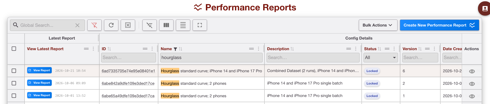
The report list provides an audit trail of generated and saved report configurations. Each row gives enough metadata to identify the report and reconstruct the analytical context. Depending on the current view, expect fields such as:

• Report name or ID: the identifier used to find the analysis later.

• Description: optional study context, for example the assay, run, validation purpose or device matrix.

• Latest report status and timestamp: the most recent generation state and time.

• Status: for example DRAFT for saved but not generated, LOCKED for generated at least once, or ARCHIVED for soft-deleted records.

• Version: the report configuration version.

• Created: the date and time the report configuration or generated report was created.

• Organisation and user identifiers: useful for audit traceability.

• Dataset identifiers: the dataset or combined dataset used for the analysis.

• Classifier and batch configuration identifiers: the qualitative and quantitative configuration versions applied during generation.

Filtering and sorting reports

Use filters to find the report you need in a long audit history. Common filters include:

• Report date: apply a from/to date range to limit the list to reports generated within a specific period.

• Qualitative classifier: filter by interpretation configuration ID.

• Quantitative batch: filter by batch or calibration configuration ID.

You can also sort by column headers, for example sorting by created date to bring the most recent analyses to the top.

Actions available

Each row includes an Actions control. You can:

• Create New Performance Report: start a new report configuration from the page header.

• View report configuration: inspect the saved settings, selected dataset, classifier, batch group, report sections, limits and version.

Bulk Actions also allow you to

• Export to Excel or CSV: download the report list metadata for administrative review.

Creating a new Performance Report

Step 1 – Describe report

Give the report a clear name and description. Good names include the assay, dataset or study purpose, and any important device or batch scope.

• Use a clear Name, for example Hourglass standard curve; iPhone 14 and iPhone 17 Pro.

• Add a Description explaining why the report is being generated, for example validation, troubleshooting, QC lot comparison or phone-matrix review.

Step 2 – Select dataset

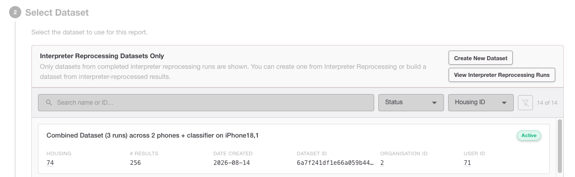
Choose the source dataset. We filter the report dataset selector to eligible non-datacollector-mode datasets and then load the classifier choices available for that dataset.

• Review dataset identifiers, run descriptions, creation dates and result counts.

• Select the dataset that matches the assay and study population you want to analyse.

• If the dataset combines multiple runs or phones, check that this is intentional and documented in the report description.

Step 3 – Dataset overview

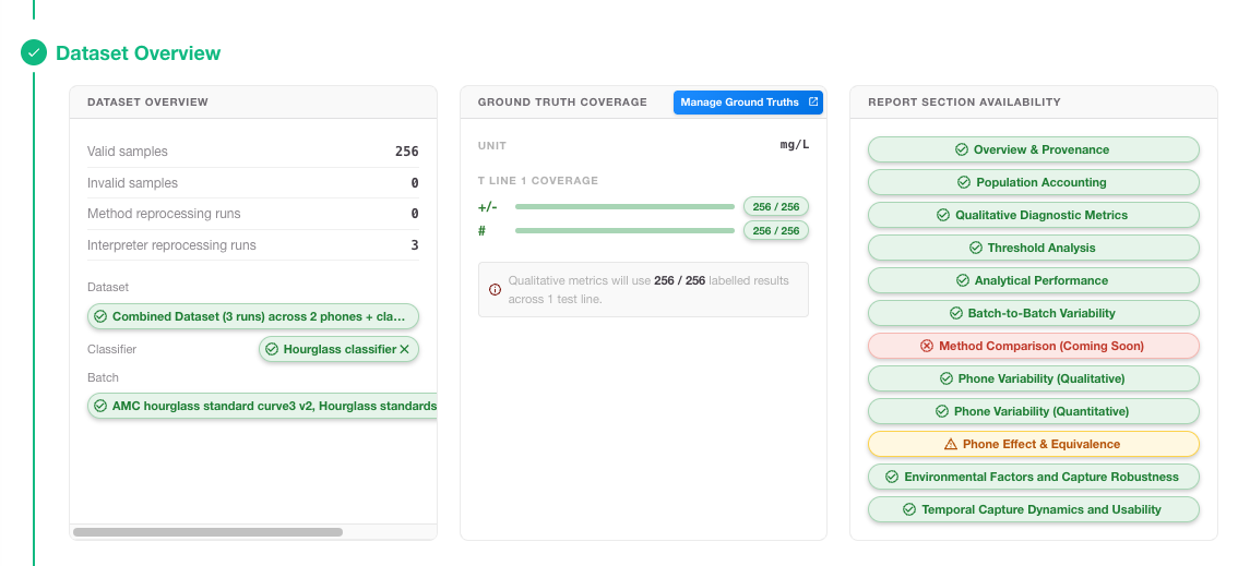
After you select the dataset, the dataset overview will show coverage and resport sections available. Confirm result counts, assay/test-line coverage, ground-truth availability and configuration compatibility.

• Total results: check that the count matches the intended study population.

• Phone model coverage: confirm whether results include one or multiple known phone models.

• Verify the Configurations (Batch and Classifier) that were used to generate these results.

• Ground truth: verify that the required qualitative classes and quantitative concentration levels are present.

Step 4 – Ground Truth Mapping

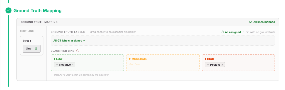
To calculate performance metrics like sensitivity and specificity, RARE needs to know which result labels correspond to your reference "Ground Truth." This mapping is flexible, allowing you to perform qualitative analysis on each specific threshold within your classifier.

Configuration Steps

• Single strip, single test line: Map the interpreter's qualitative bins (e.g., "Positive", "Negative") to the Ground Truth categories.

• Multiple strips / multiple test lines: For complex assays, ensure each test line is correctly mapped to its respective reference standard.

• The system will validate that the mapping is complete before allowing you to move to the next step.

Mapping Multi-Bin Classifiers

If your classifier uses multiple bins (e.g., Low, Medium, and High), you can generate reports for different clinical scenarios by grouping these bins against your Ground Truth. This is achieved by mapping the thresholds between the bins:

• Scenario A (Low vs. Others): You can map the first threshold so that Low is compared against a combined group of Medium + High.

• Scenario B (High vs. Others): You can map the second threshold so that Low + Medium are grouped together and compared against High.

Step 5 – Choose report sections and limits

Customize your report by selecting the specific analysis modules you need. You can toggle these on or off based on your validation requirements:

The Portal supports a presentation density setting, for example a compact executive/triage view or a fuller regulatory/DHR view with expanded tables and matrices.

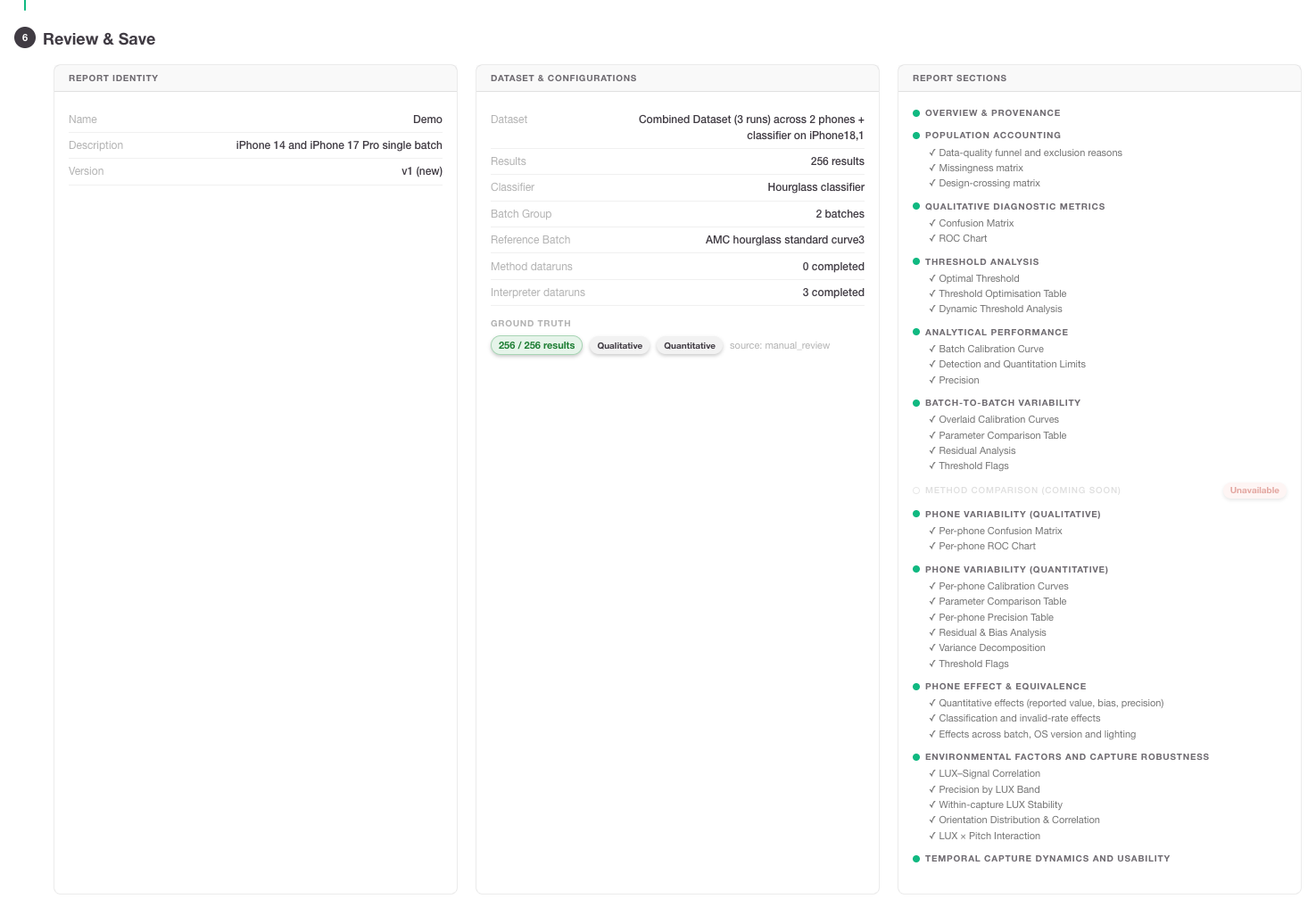
Step 6 – Review, save and generate

Review the configuration summary, then save and generate the report.

• Check the report name, dataset, classifier, batch group, ground-truth mapping, selected sections, density and limits.

• Click Save Configuration to store the settings and create a versioned configuration.

• Click Generate Report to start the calculation engine.

• For large datasets or reports with phone-specific fitting and temporal plots, allow additional processing time.

Interpreting a generated report

A generated report should be read from scope to conclusion:

first confirm what data was included, then review population completeness, then interpret each analytical module. Avoid reading a single chart without checking denominators, exclusions, unavailable states and section limitations.

Report contents and PDF export

The PDF export is an expanded, paginated view of the generated report with running headers and a table of contents.

• Use Export PDF from the report view to create an offline record for review, sharing or filing.

• Sections switched off in the report configuration retain their number and are listed as not included.

• Sections switched on but not computable report unavailable or not-estimable states rather than silently omitting the problem.

• Temporal plots in PDF may reflect the active report view selection and may use reproducible sampling for dense frame data; check the reported counts and sampling disclosures.

Using exported XLS or other tabular exports for further analysis

When you need deeper analysis than the report view provides, export the underlying or summary tables where available. In a spreadsheet or statistics package, useful follow-up checks include:

• Reconcile denominators: compare section-level counts with the population funnel and missingness matrix before drawing conclusions.

• Filter by phone, batch and concentration: inspect whether apparent phone differences are really caused by uneven concentration or batch distribution.

• Investigate sparse cells: treat phone × batch × concentration cells with fewer than three observations as exploratory, not definitive.

• Plot residuals and CV by concentration: a global CV can hide concentration-specific instability near LoD or at the top of the range.

• Review telemetry coverage: environmental conclusions are weak if lux/orientation data are missing for many records or concentrated in only one phone or batch.

• Keep identifiers: retain report ID, dataset ID, result IDs, phone model, batch ID, classifier version and configuration version in any downstream workbook so that analyses remain traceable.

Report section guide

1 · Provenance & Scope

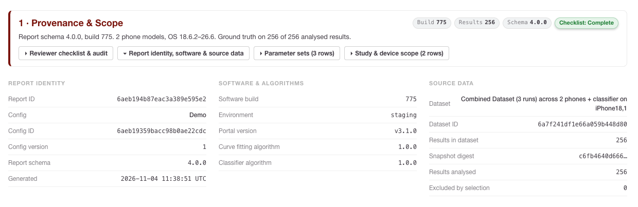
This section is the report’s technical passport. It records the organisation, generated-by user, generated-on timestamp, RARE Portal version, dataset scope, test-line scope, phone-model scope, profile/configuration identity and calculation timestamp.

Use it to answer:

• Was the report generated in the expected environment, for example RARE Portal v3.1.0?

• Does the dataset ID match the validation or QC study you intended to review?

• Which phone models, test lines, classifier split and profile version were included?

• Is the calculation timestamp appropriate, or could the dataset have changed between selection and generation?

1.1 · Population Accounting

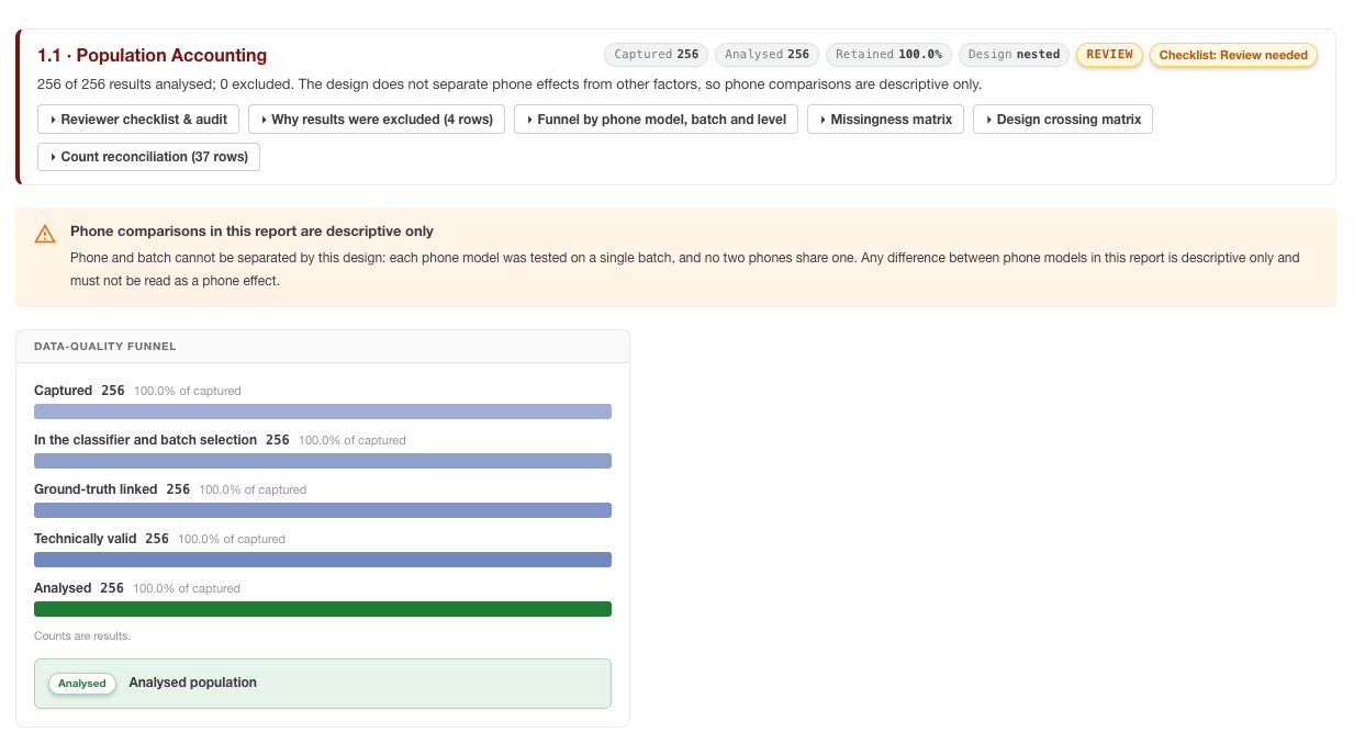
Population Accounting was added to make the analysed population auditable.

It includes:

• Data-quality funnel: Captured → In the classifier and batch selection → Ground-truth linked → Technically valid → Analysed.

• Exclusion reasons: selection exclusions, missing ground truth, invalid captures and missing analysis signal.

• Missing result documents: represented separately as not_found, not as an ordinary exclusion reason.

• Missingness matrix: missing counts, percentages and denominators for fields such as signals, ground truth, image, capture status, lux and orientation.

• Design-crossing matrix: phone × batch × concentration or class counts, including zero-count cells and sparse-cell flags.

Spreadsheet follow-up: Pivot the exported data by phone model, batch and concentration/class. Look for empty or sparse combinations and confirm whether every section uses the same denominator for the same filter selection.

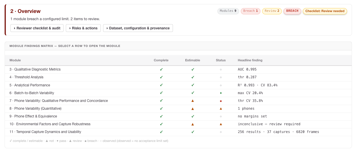
2 · Overview

The Overview gives a high-level summary of report findings and section states. Use it for triage, not as a replacement for detailed section review.

3 · Qualitative Diagnostic Metrics

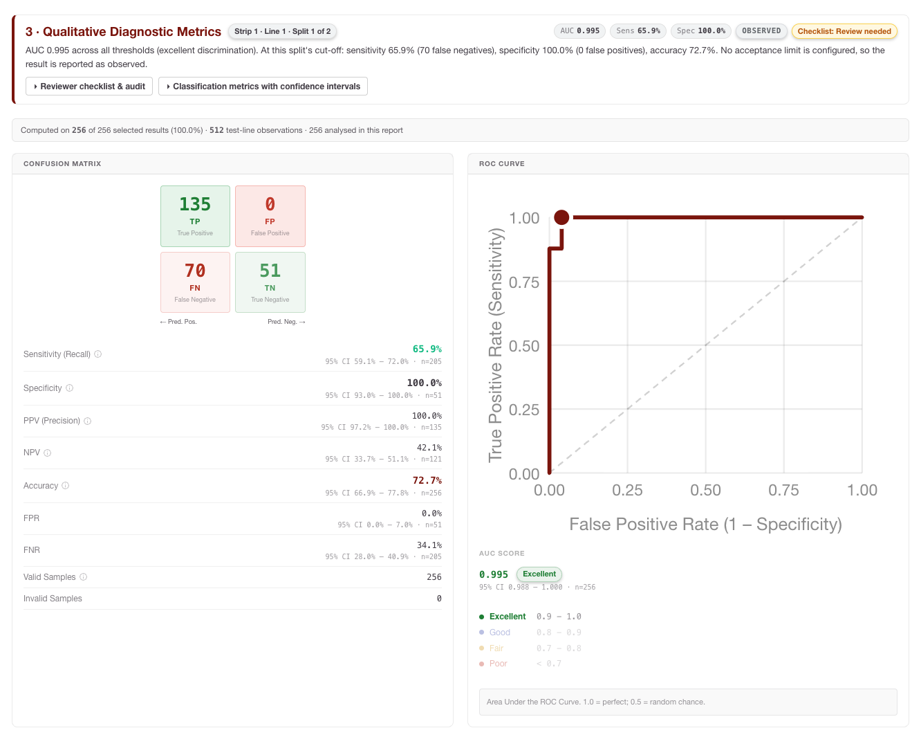
This section compares classifier calls with ground-truth classes for the selected test line and classifier split.

These equations evaluate the interpreter’s qualitative classifications against assigned Ground Truth reference classes (TP = True Positive, TN = True Negative, FP = False Positive, FN = False Negative).

Sensitivity (Positive Percent Agreement - PPA)

The proportion of actual positive samples that are correctly identified by the interpreter. It measures the assay's ability to avoid false negatives.

Specificity (Negative Percent Agreement - NPA)

The proportion of actual negative samples that are correctly identified by the interpreter. It measures the assay's ability to avoid false positives.

Positive Predictive Value (PPV)

The probability that a sample identified as positive by the interpreter is truly positive. This indicates the reliability of a positive result.

Negative Predictive Value (NPV)

The probability that a sample identified as negative by the interpreter is truly negative. This indicates the reliability of a negative result.

Overall Accuracy

The proportion of all samples (both positive and negative) that were correctly identified by the interpreter.

Spreadsheet follow-up: Recalculate metrics by site, run, batch, phone or concentration band to see whether the pooled result masks a subgroup problem.

4 · Threshold Analysis

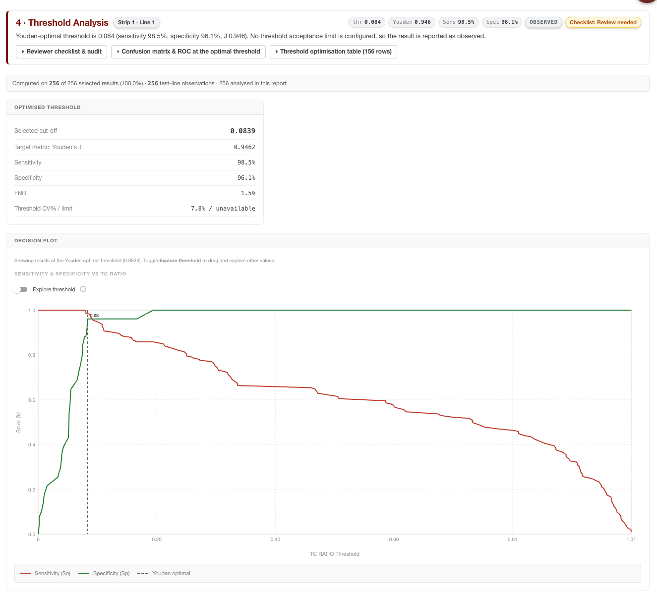
Threshold Analysis shows how classifier performance changes when the decision threshold moves. It typically includes ROC curves, AUC, threshold optimisation, Youden’s Index and decision plots.

ROC (Receiver Operating Characteristic) Curves

A visual representation of the trade-off between Sensitivity and Specificity. The curve plots the True Positive Rate against the False Positive Rate at various threshold settings. The Area Under the Curve (AUC) is also calculated, providing a single global metric for the interpreter's ability to discriminate between positive and negative samples.

Threshold Optimization Table

A detailed breakdown showing how specific diagnostic metrics (Sensitivity, Specificity, PPV, NPV) would shift if you moved your threshold up or down. This allows you to select a cut-off that prioritizes the specific clinical needs of your assay (e.g., maximizing sensitivity for a screening test).

Youden’s Index

To assist in identifying the mathematically "optimal" threshold, RARE calculates Youden’s Index for every point on the ROC curve. This index represents the point where the sum of Sensitivity and Specificity is maximized.

Decision Plot

In addition to the optimization table, the Decision Plot provides a powerful visual summary of your assay's performance across the entire threshold range. This dual-axis chart plots both Sensitivity and Specificity simultaneously against the threshold value.

The Decision Plot allows you to:

• Identify the Crossover Point: Easily locate the "Equal Error Rate" where Sensitivity and Specificity intersect, representing a balanced performance profile.

• Visualize Performance Trade-offs: See at a glance how rapidly Sensitivity drops or Specificity rises as you adjust your cut-off, helping you identify "stable" regions where minor variations in signal won't drastically impact clinical results.

• Support Clinical Justification: By overlaying these two critical metrics, the plot provides a clear visual rationale for selecting a specific threshold—for example, choosing a point slightly to the left of the intersection to prioritize high Sensitivity for a screening application.

This graphical representation transforms the raw data of the optimization table into an intuitive tool for making informed, data-driven configuration decisions.

Spreadsheet follow-up: Export threshold tables and mark candidate thresholds that preserve acceptable sensitivity/specificity over a stable range rather than at a single sharp peak.

5 · Analytical Performance

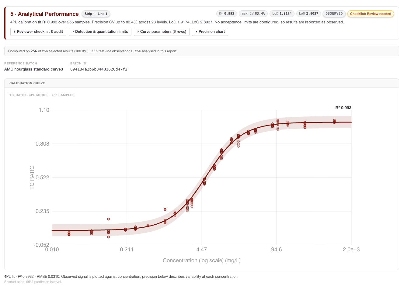
Analytical Performance evaluates the quantitative response. Depending on the configuration and dataset, it can include standard-curve fit, LoD, LoQ, linearity/regression, bias, recovery and precision.

• LoD: the lowest signal or concentration distinguishable from background using the configured statistical approach.

• LoQ: the lowest concentration that can be quantified with acceptable precision and accuracy.

Linearity and Regression Analysis

This module compares the interpreter's quantitative output against the expected Ground Truth values. RARE generates a scatter plot with a Linear Regression line to visualize the relationship. Key statistics provided include the Slope, Intercept, and the Coefficient of Determination , which indicates how well the data fits the linear model, where and

Bias and Recovery

This analysis determines if the system consistently over- or under-estimates concentrations. RARE calculates the Percent Recovery for each sample, providing a clear view of systematic error across different concentration levels.

Precision (Repeatability)

By analyzing replicates within your dataset, RARE evaluates the "closeness of agreement" between independent results. This is expressed as the Coefficient of Variation (%CV), a standardized measure of dispersion that allows you to assess the stability of your assay and interpreter across multiple runs.

where is the standard deviation and is the mean of the replicates.

Spreadsheet follow-up: Plot residuals by concentration and batch. Compare CV% near the clinical threshold with CV% at high concentrations; the threshold-adjacent region is often more important for classification reliability.

6 · Batch-to-Batch Variability

Batch-to-Batch Variability section provides the critical evidence needed to demonstrate the robustness of your interpreter across different manufacturing lots. In lateral flow production, slight variations in materials or reagent deposition can impact signal intensity; This section compares calibration behaviour across manufacturing lots or batch configurations. It can include curve overlays, parameter comparison tables and residual distributions.

Based on the analysis modules, this section includes:

• Calibration Curve Overlay: This plot displays the mathematical fit for each batch configuration included in the report. By overlaying these curves, you can visually assess if different lots follow the same response trajectory or if there is a "shift" in signal intensity across the concentration range.

• Parameter Comparison Table: RARE extracts the key coefficients from the underlying 4PL or 5PL models (such as Slope, EC50, and Asymptotes) and presents them side-by-side. This allows you to quantify exactly how the biochemical response varies between lots.

• Residuals (Observed - Predicted) Box Plot: This diagnostic tool visualizes the distribution of error for each batch. It helps you identify if a specific lot has a higher degree of "noise" or a consistent bias compared to the others.

Spreadsheet follow-up: Pivot residuals and recovery by batch and concentration. If one batch differs mainly at low concentration, the practical impact may be different from a whole-curve shift.

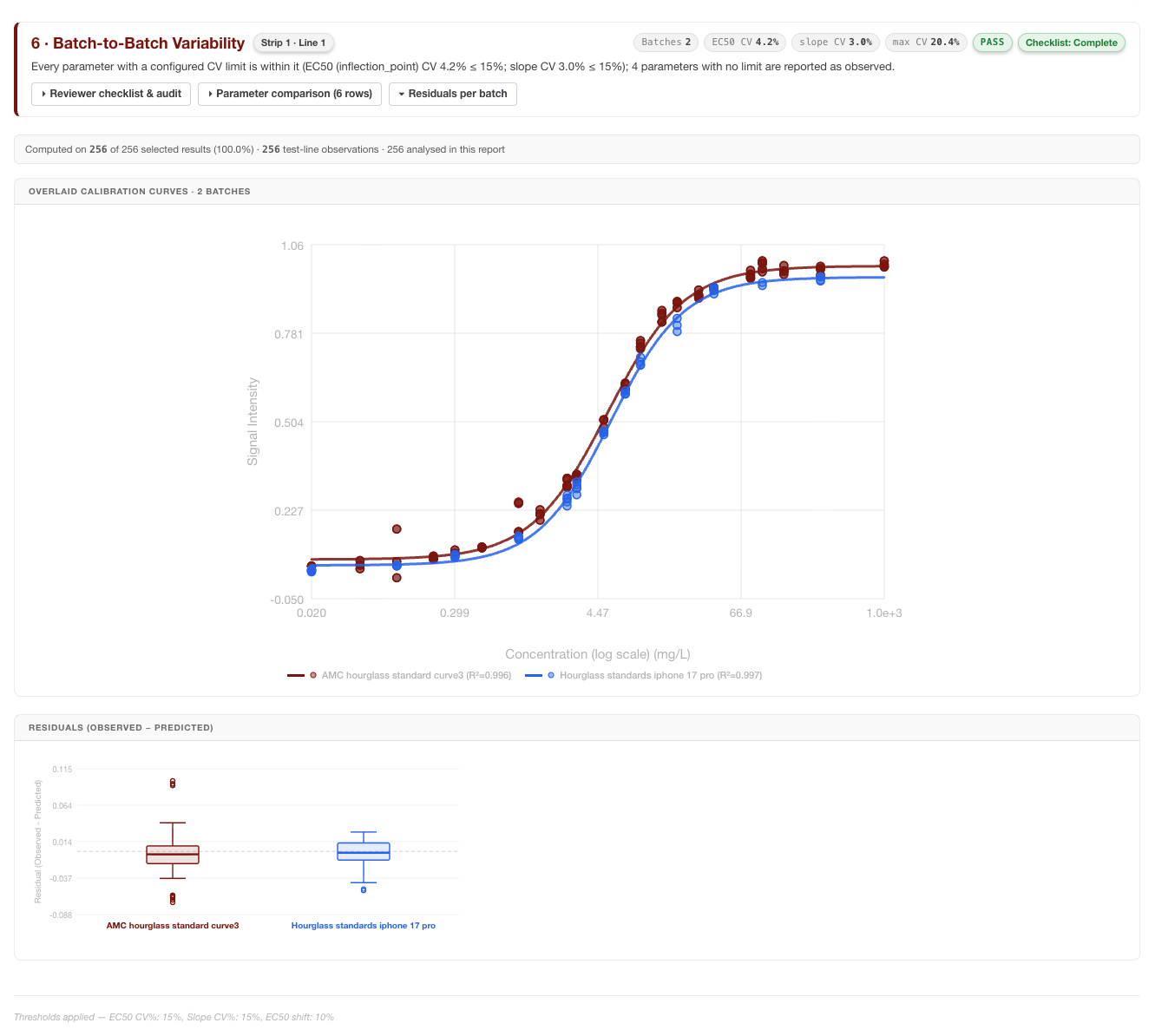
Understanding the Residuals Box Plot

The box plots in this section allow you to see at a glance how consistently each batch is performing. For each batch:

• The Center Line (Median): Represents the median residual. If this line is at zero, the batch is perfectly centered on the Ground Truth. If it is consistently above or below zero, it indicates a systematic bias for that specific lot.

• The Box (Interquartile Range - IQR): Represents the middle 50% of your data. A "taller" box indicates higher variability (lower precision) within that batch.

• The Whiskers: Extend to show the spread of the rest of the data.

• Outliers (Individual Dots): Any results that fall significantly outside the expected range are plotted as individual points, helping you identify specific samples that may have had physical defects or interpretation anomalies.

Batch Comparison Metrics

RARE calculates how each "Test" batch deviates from the designated Reference Batch using the following formulae:

Mean Residual (Bias):
The average difference between the measured values and the Ground Truth for the batch.

Batch-Specific Coefficient of Variation (%CV):
This metric quantifies the precision of the residuals for a specific batch, allowing you to compare the "tightness" of results against your reference lot.

By analyzing these plots and tables, you can objectively determine if a new manufacturing lot is performing within your established QC tolerances or if it requires a unique calibration update.

7 · Phone Variability: Qualitative Performance and Threshold Stability

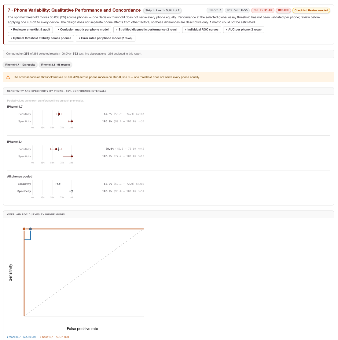
This section reports diagnostic classification performance separately by smartphone model. It includes per-phone confusion matrices, sensitivity, specificity, accuracy, PPV, NPV, false-positive rate and false-negative rate, with denominators and 95% confidence intervals where estimable. It can also show per-phone ROC curves, AUC with confidence intervals and Youden-optimal threshold stability.

The section is available when a classifier has been applied and at least two known phone models each have enough ground-truth results. Smaller additional groups may be shown but do not necessarily support every metric.

Spreadsheet follow-up: Export per-phone metrics and review FN/FP counts by concentration or signal band. Investigate whether one phone is overrepresented near the threshold, because that can magnify apparent diagnostic differences.

8 · Phone Variability (Quantitative)

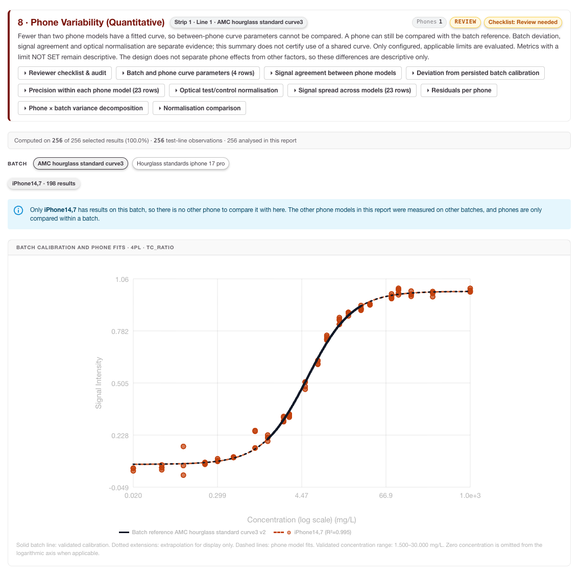
This section evaluates quantitative signal behaviour by phone model within each batch and test line. It may include independent 4PL, 5PL or linear fits per phone, curve overlays, parameter summaries, concentration-level mean/SD/CV%, residual summaries, variance components and comparisons with the selected batch calibration reference.

Spreadsheet follow-up: Plot signal, T/C ratio and residuals by phone and concentration. Compare before/after or processed-signal versus T/C-ratio CV where available, but do not treat a CV reduction as validation of a deployed correction unless that study was explicitly designed and controlled.

9 · Phone Effect & Equivalence

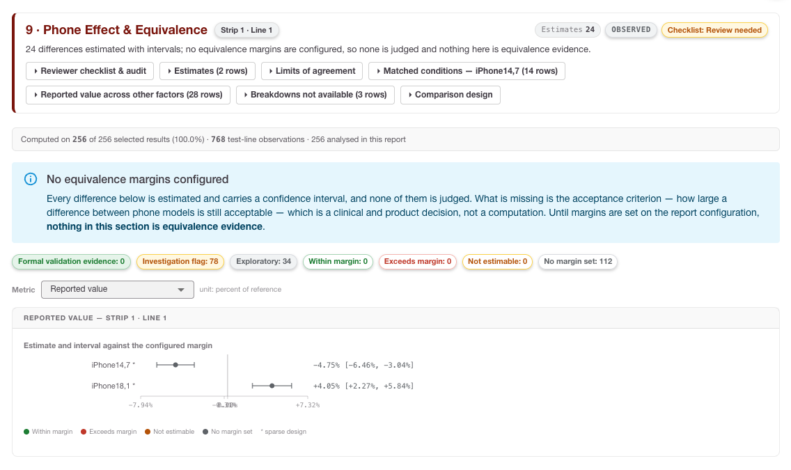
This section calculates phone-model effect estimates against either a configured reference phone model or the other phone models pooled. It reports the estimate, units, sample counts, 95% confidence interval and comparison with saved lower and/or upper metric bounds.

Status values may include:

• within_margin: the reported interval lies within the configured numerical bounds.

• exceeds_margin: the estimate or interval crosses a configured bound.

• not_estimable: the estimate or interval cannot be calculated.

• not configured: no applicable margin was saved before report generation.

Spreadsheet follow-up: Recreate forest-plot tables and flag comparisons with sparse counts, one-sided margins, disjoint batches or unresolved not-estimable rows. Use these flags to plan a better crossed phone × batch × concentration study if formal equivalence evidence is needed.

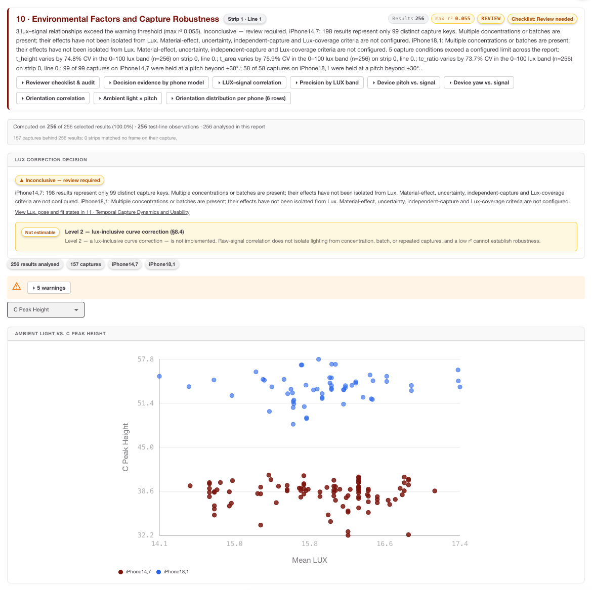
10 · Environmental Factors and Capture Robustness

This section explores associations between capture conditions and signal measurements. It can include lux versus signal plots, pitch/yaw versus signal plots, Pearson and Spearman correlations, lux-banded precision and counts of excluded records without usable telemetry.

Spreadsheet follow-up: Export telemetry and signal fields, then stratify by concentration, batch and phone before interpreting a lux or orientation trend. If a high-lux band appears worse, check whether it also contains a different phone or batch mix.

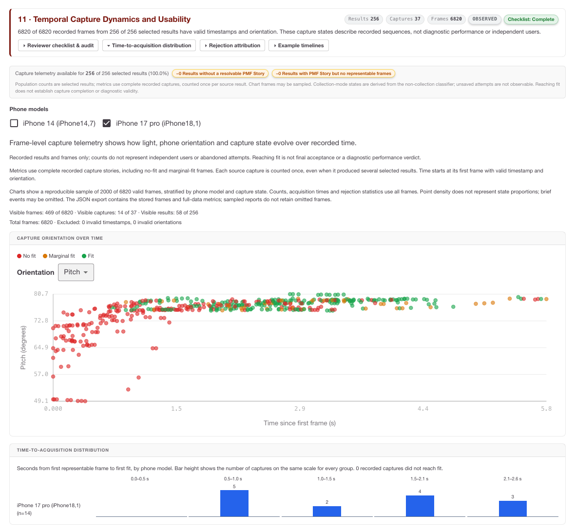
11 · Temporal Capture Dynamics and Usability

This section uses PMF story timing and telemetry to visualise capture dynamics. It can show frame state, orientation and lux over capture time, along with capture identity, telemetry provenance, selected result counts, distinct capture counts and frame counts.

Spreadsheet follow-up: For usability investigations, group frames by capture ID and compare duration, frame count, fit state, pitch/yaw variation and lux variation. Avoid treating every frame as an independent sample when it comes from the same capture story.

Calibration fitting failures and inspection

When a recognised fit failure occurs, the report should isolate the failure to the affected phone model or analysis slice, preserve independent outputs, and mark fit-dependent outputs as unavailable with a reason.

If underlying calibrator concentration-versus-signal points are available, the user can inspect them as a scatter plot without a fitted curve. This helps distinguish data-quality or concentration-response anomalies from transport or request errors.

Viewing or editing an existing report configuration

Open an existing report configuration when you need to inspect settings, regenerate a report or create a new version.

• View report: opens the generated report view for metrics, charts and result breakdowns.

• Save as a new version: use this when you need to change dataset, classifier, batch group, sections or limits while preserving the previous configuration.

• Generate or regenerate: runs the analysis using the saved settings.

• Verify lineage: confirm the configuration version, dataset ID, classifier version, batch version and RARE Portal version before using results in a validation or QC record.

After generating a report

After a report is generated:

• Start with scope: verify provenance, dataset, test-line, classifier split, phone models and generation time.

• Review population accounting: ensure analysed counts, missingness and sparse design cells support the intended interpretation.

• Read section limitations: especially for phone equivalence, environmental analysis and temporal usability outputs.

• Export the PDF: keep a human-readable record with charts, tables, contents and running headers.

• Export tables where available: use spreadsheet analysis to investigate denominators, outliers, sparse cells and subgroup effects.

• Protect data integrity: report generation does not rewrite original stored measurements; it creates an analysis snapshot from selected data and configuration versions.

Appendices

The following appendices provide the proposed calculation models for the report sections added or expanded for population accounting, phone variability, phone-effect margin comparison, environmental robustness and temporal usability. They are intended to make the report calculations transparent for LF manufacturing, QC and laboratory users, and to support independent review in exported tabular data where those fields are available.

Appendix A · Section 1.1 Population Accounting calculations

Funnel stage yield and overall retention

For each population-accounting stage:

Overall retention from capture to analysis is:

Where: N_k is the record count at funnel stage k, for example Captured → Selected → Ground-truth linked → Technically valid → Analysed.

Spreadsheet check: =(CurrentStageCount / PreviousStageCount) * 100

Field-level missingness rate

Where: M_j is the missingness rate for field j, such as ground truth, signal, image, capture status, lux, pitch or yaw.

Spreadsheet check: =(MissingFieldCount / TotalRecordCount) * 100

Design-crossing sparse-cell flag

Where: N_ijk is the number of records in a phone model × batch × concentration or class cell.

Spreadsheet check: =IF(CellCount<3,"Sparse cell","OK")

Appendix B · Section 7 Phone Variability: Qualitative Performance and Threshold Stability calculations

Per-phone false-positive and false-negative rates

Where: subscript p denotes a specific phone model. TP, TN, FP and FN are counted separately for that phone.

Spreadsheet check: =FP/(TN+FP) and =FN/(TP+FN)

Wilson score confidence interval for proportions

Where: p̂ is the observed proportion, such as sensitivity, specificity or accuracy; n is the relevant denominator; and z = 1.96 for an approximate 95% confidence interval.

Optimal-threshold instability across phone models

Where: T_opt,p is the Youden-optimal threshold calculated independently for phone model p, and P is the number of phone models.

Spreadsheet check: =(STDEV.S(threshold_range)/AVERAGE(threshold_range))*100

Appendix C · Section 8 Phone Variability (Quantitative) calculations

Four-parameter logistic standard curve

Five-parameter logistic standard curve

Where: x is analyte concentration; y is optical density, peak height or T/C ratio; a is the minimum asymptote; d is the maximum asymptote; c is the inflection concentration or EC50; b is the slope parameter; and g is the asymmetry parameter. When g = 1, the 5PL model reduces to a symmetric 4PL form.

Concentration-specific residual relative to a reference curve

Where: y_p,k is the observed response for phone p at concentration x_k, and ŷ_ref(x_k) is the predicted response from the selected reference batch or reference calibration curve.

Spreadsheet check: =ObservedResponse - ReferencePredictedResponse

Appendix D · Section 9 Phone Effect & Equivalence calculations

Estimated phone-model effect

The same structure may be used when the comparison is against the pooled mean of the other phone models, depending on the report configuration.

Standard error of the difference

Where: s_test and s_ref are the standard deviations for the test and reference phone groups, and n_test and n_ref are their sample counts.

Spreadsheet check: =SQRT((STDEV.S(test_range)^2/COUNT(test_range))+(STDEV.S(ref_range)^2/COUNT(ref_range)))

Confidence interval for the effect estimate

Where: t_(1-α,ν) is the Student t critical value and ν is the applicable degrees of freedom, often using a Welch/Satterthwaite approximation when variances differ.

Margin comparison decision rule

Where: -θ_L and +θ_U are the configured lower and upper acceptance margins.

Appendix E · Section 10 Environmental Factors and Capture Robustness calculations

Pearson correlation coefficient

Where: E_i is an environmental parameter, such as lux, pitch or yaw, and y_i is the signal or T/C ratio.

Spreadsheet check: =CORREL(environment_range, signal_range)

Spearman rank correlation

Where: d_i is the difference between the rank of the environmental value and the rank of the signal value for observation i.

Lux-banded precision

Where: observations are grouped into lux brackets, for example low, medium and high lux, and s_tier is the standard deviation within a tier at a fixed concentration or other controlled stratum.

Spreadsheet check: =(STDEV.S(tier_signal_range)/AVERAGE(tier_signal_range))*100

Appendix F · Section 11 Temporal Capture Dynamics and Usability calculations

Purpose: Use these calculations to describe capture timing, orientation stability and frame-fit behaviour from PMF story or frame telemetry. These are capture-dynamics metrics, not a complete measure of abandoned attempts or independent user behaviour unless those data are explicitly recorded.

Total capture duration or lock time

Spreadsheet check: =FinalLockTimestamp - FirstFrameTimestamp

Combined angular tilt

Spreadsheet check: =SQRT(Pitch^2 + Yaw^2)

Frame-fit stability rate

Spreadsheet check: =(ValidFrameCount / TotalFrameCount) * 100